Some evidence or verbal trick to illustrate the potential of quantum applications.

• Though in their infancy, the stability of qubits should become much better over time. -- IBM
• As IBM’s quantum hardware scales rapidly – from small prototype systems to more promising larger devices – researchers are excited about the possibility to one day handle previously insoluble routing problems.
• “A glimpse of the quantum future”
• As the hardware matures according to goals laid out in IBM Quantum’s hardware roadmap, the researchers expect to demonstrate a clear advantage over the classical competition.

Refs

1. https://qiskit.org/textbook/ch-machine-learning/machine-learning-qiskit-pytorch.html#Contents
2. https://qulearn.baidu.com/textbook/chapter5/%E9%87%8F%E5%AD%90%E5%88%86%E7%B1%BB%E5%99%A8.html

Brief

1. Classical data $\to$ quantum states (quantum data).
2. Quantum Variational Circuit (QPU)
3. Measure output and compute loss

Case: Quantum Chemistry with Qu&Co’s (now Pasqal) QUBEC on Amazon Braket

"To set expectations correctly, so far, no variational quantum algorithm has outperformed classical supercomputers in computational chemistry based on first principles (ab initio). However, recently quantum advantage has been demonstrated on a theoretical sampling task,[4] and an increasing number of academic and industrial works are bringing down the resource requirements, devising better quantum circuit strategies and more efficient optimization protocols. The race is on, and many believe chemistry or materials science applications to be one of the candidates to show early examples of industry relevant quantum advantage on near-term hardware."

• Evaluating the evidence for exponential quantum advantage in ground-state quantum chemistry (Nature-Comm 2023, CalTech)

Reference: https://qml.baidu.com/tutorials/quantum-simulation/hamiltonian-simulation-with-product-formula.html

According to one of the fundamental axioms of quantum mechanics, the evolution of a system over time can be described by $$ i\hbar\frac{\delta}{\delta t}|\psi\rangle = H|\psi\rangle $$ $\hbar$ is the reduced Planck constant. This equation is the well-known Schrödinger equation. Thus, for a time independent Hamiltonian, the time evolution equation of the system can be written as $$ |\psi(t)\rangle = U(t)|\psi(0)\rangle, U(t) = e^{-iHt} $$ Here we take the natural unit $\hbar = 1$ and $U(t)$ is the time evolution operator. The idea of simulating the time evolution process with quantum circuits is to approximate this time evolution operator using the unitary transformation constructed by quantum circuits.

Sample Question

For the Hamiltonian $H = I\otimes X + 0.5I\otimes Z - 0.2X\otimes X + 1.2Z\otimes I + 0.5Z\otimes Z$, find a quantum circuit $U$ to simulate $e^{-iH}$ with error tolerance 0.01 (i.e., $||U - e^{-iH}||\leq 0.01$). Moreover, try to use the idea of variational quantum circuit compiling to simplify the circuits.

• A Quantum Approximate Optimization Algorithm

Intro from Huawei Mindspore

qaoa-maxcut

qaoa

"It is important to say that, given the classical nature of combinatorial problems, exponential speedup in using quantum computers compared to the best classical algorithms is not guaranteed."

Intro from Baidu

Consists of $n$ bits and $m$ clauses. Each clause ( $C$ ) is a constraints for part of bits. Here $z$ represents the bit series $z_{1} z_{2} \dots z_{n}$

$$ C_j(z) = \begin{cases} 1 & \text{if clause $j$ is satisfied} \\ 0 & \text{if clause $j$ is not satisfied} \end{cases} $$

We have the objective function:

$$ C(z) = \sum_{j=1}^{m}{w_j C_j(z)} $$

Objective: find $z$ that maximize $C(z)$

"对于一个问题，如果我们找到了它的哈密顿量，根据这个哈密顿量我们可以求得它的本征态和本征能量，得到了本征态和本征能量就相当于解决了这个问题" -- 本源量子视频

Transform to an optimization problem on quantum system. Consider a compute basis $|z\rangle \in \lbrace0,1\rbrace^n$.

Define the Hamiltonian as:

$$ H_{C_j}|z\rangle = C_j(z)|z\rangle $$

Where the Hamiltonian can be constructed as:

$$ H_{C_j} = \sum_{z\in {0,1}^n}{C_j(z)|z\rangle \langle z|} $$

Why?

$$ \langle z'| z\rangle = \begin{cases} 1 & \text{if } z' = z \\ 0 & \text{else} \\ \end{cases} $$

So $\sum_{z'\in {0,1}^n}{C_j(z')|z'\rangle \langle z'|} z\rangle = C_j(z)|z\rangle$

For example, consider we have $z^{(1)}$ and $z^{(2)}$ that satisfy $C_j$, the the Hamiltonian is:

$$ H_{C_j}=|z^{(1)}\rangle \langle z^{(1)}|+| z^{(2)}\rangle \langle z^{(2)}| . $$

To this end, QAOA encodes the objective function $C$ into a $n$-Qubit quantum system's Hamiltonian.

$$ H_C=\sum_{j=1}^m w_j H_{C_j}, $$

Which satisfy the eigen equation:

$$ H_C|z\rangle=\sum_{j=1}^m w_j H_{C_j}|z\rangle=\sum_{j=1}^m w_j C_j(z)|z\rangle=C(z)|z\rangle $$

Notice that, assume the optimal solution is $z_{\text{opt}}$, we have:

$$ \left\langle z_{\mathrm{opt}}\left|H_C\right| z_{\mathrm{opt}}\right\rangle=\left\langle z_{\mathrm{opt}}\left|C\left(z_{\mathrm{opt}}\right)\right| z_{\mathrm{opt}}\right\rangle=C\left(z_{\mathrm{opt}}\right)\left\langle z_{\mathrm{opt}} \mid z_{\mathrm{opt}}\right\rangle=C\left(z_{\mathrm{opt}}\right) $$

Thus the optimal solution is the eigenvector of the Hamiltonian with the maximum eigenvalue ( $C_{max}$ )

For arbitrary quantum state $\psi$, we have:

$$ \langle \psi | H_C |\psi \rangle \leq C(z_{\text{opt}}) $$

Why? Because:

$$|\psi \rangle = \sum_i^n{c_i|z_i\rangle}, \sum_i^n{|c_i|^2} = 1$$

Therefore:

$$ \begin{aligned} \langle \psi | H_C |\psi \rangle &= \sum_{i}^{n}{c_i^* \langle z_i|} H_C \sum_{i}^{n}{c_i|z_i\rangle} \\ &= \sum_{i}^{n}{c_i^* \langle z_i|}\sum_{i}^{n}{c_i H_{C}|z_i\rangle} \\ &= \sum_{i}^{n}{c_i^* \langle z_i|}\sum_{i}^{n}{c_i C(z_i)|z_i\rangle} \\ &= \sum_{i}^{n}{C(z_i) c_i^*c_i \langle z_i|z_i \rangle} \\ &= \sum_{i}^{n}{|c_i|^2 C(z_i)} \\ &\leq \sum_{i}^{n}{|c_i|^2 C(z_{\text{opt}})} = C(z_{\text{opt}}) \end{aligned} $$

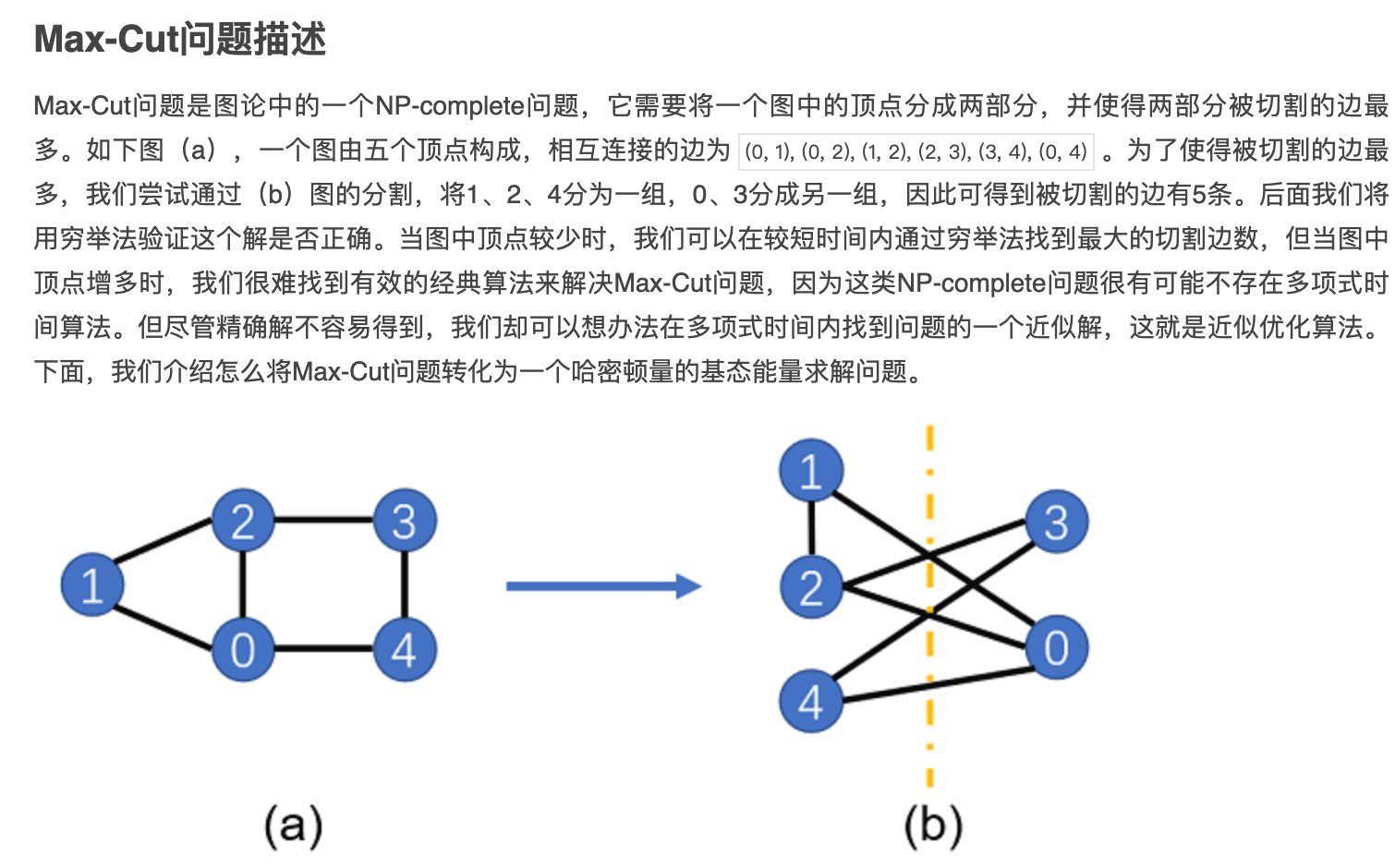
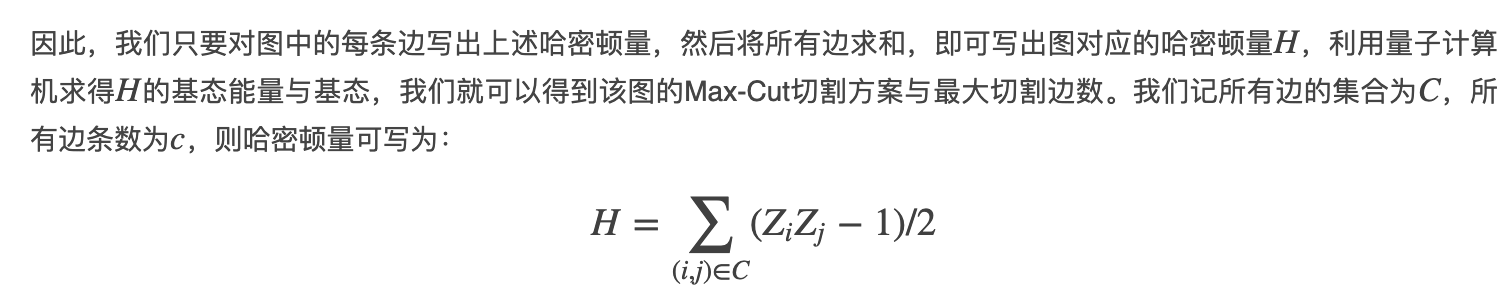
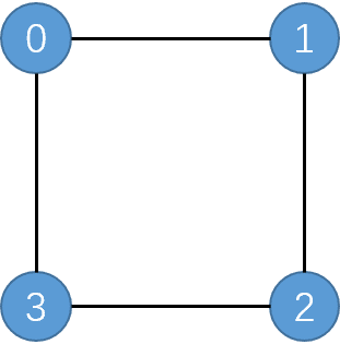
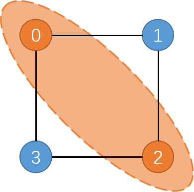
For a graph $G = (V,E)$, we have $n = |V|$ vertexes and $m = |E|$ edges. For each vertex $v$ in $G$, the value $z_v$ is 0 or 1 (0, 1 represent two partitions). For each edge $E = (u,v)$. A "clause" requires that $z_u \neq z_v$, meaning that vertex $v$ and $u$ are divided into different sub-sets. For each edge in the graph we have (XOR):

$$ C_(u,v)(z) = z_u + z_v - 2z_u z_v $$

Note that only $z_u \neq z_v$ results in 1, otherwise 0.

The entire problem is:

$$ C(z) = \sum_{(u,v)\in E}{C_(u,v)(z)}=\sum_{(u,v)\in E}{z_u + z_v - 2z_u z_v} $$

Hamiltonian $$ Z\equiv \begin{bmatrix} 1 & 0 \ 0 & -1 \end{bmatrix} \ Z|0\rangle = |0\rangle \ Z|1\rangle = -|1\rangle $$

Using $Z$ gate to construct Hamiltonian of the system. (Use mapping: $f(x)\rightarrow\frac{1-x}{2}$)

$$ \begin{aligned} H_C &= \sum_{(u,v)\in E}{C_(u,v)(z)} = \sum_{(u,v)\in E}{\frac{I-Z_u}{2} + \frac{I-Z_v}{2} - 2 \frac{I-Z_u}{2} \frac{I-Z_v}{2}} \\ &= \sum_{(u,v)\in E}{\frac{2I - Z_u - Z_v - (Z_u Z_v - Z_u - Z_v + I)}{2}} \\ &= \sum_{(u,v)\in E}{\frac{I - Z_u Z_v}{2}} \end{aligned} $$

Why? $$ \begin{aligned} H_C |z\rangle &= \sum_{(u,v)\in E}{\frac{I - Z_u Z_v}{2} |z\rangle} \ &= \sum_{(u,v)\in E}{\frac{|z_0\rangle \otimes \cdots \otimes (I - Z_u Z_v) |z_u z_v\rangle \otimes \cdots \otimes |z_n\rangle }{2}} \end{aligned} $$

Note that (according to equition 71):

$$ Z_u Z_v |z_u z_v\rangle = \begin{cases} -|z_u z_v\rangle & \text{if } z_u \neq z_v \\ |z_u z_v\rangle & \text{if } z_u = z_v \end{cases} $$

Here

$$ \begin{aligned} Z_u Z_v | z_u z_v \rangle &\equiv (Z_u \otimes Z_v) (z_u \otimes z_v) \\ &= Z_u|z_u\rangle \otimes Z_v|z_v\rangle \end{aligned} $$

Thus:

$$ \frac{|z_0\rangle \otimes \cdots \otimes (I - Z_u Z_v) |z_u z_v\rangle \otimes \cdots \otimes |z_n\rangle }{2} = \begin{cases} |z\rangle & \text{if } z_u \neq z_v \\ 0 & \text{if } z_u = z_v \end{cases} $$

Therefore

$$ \begin{aligned} H_C |z\rangle = \sum_{(u,v)\in E}{(z_u + z_v - 2z_u z_v)|z\rangle} \end{aligned} $$

The expectation of $H_C$ with state $\psi$ is: $$ \begin{aligned} \langle\psi|H_C| \psi\rangle &=\langle\psi|\sum_{(u, v) \in E} \frac{I-Z_u Z_v}{2}| \psi\rangle \ &=\langle\psi|\sum_{(u, v) \in E} \frac{I}{2}| \psi\rangle-\langle\psi|\sum_{(u, v) \in E} \frac{Z_u Z_v}{2}| \psi\rangle \ &=\frac{|E|}{2}-\frac{1}{2}\langle\psi|\sum_{(u, v) \in E} Z_u Z_v| \psi\rangle . \end{aligned} $$

Denote $H_D = -\sum_{(u, v) \in E} Z_u Z_v$, we need find $|\psi\rangle$ to maximize $\langle \psi| H_D | \psi \rangle$

$$ U_B\left(\beta_p\right) U_D\left(\gamma_p\right) \cdots U_B\left(\beta_1\right) U_D\left(\gamma_1\right), $$

Tune $\beta$ and $\gamma$ to find the optimal $| \psi (\beta, \gamma)\rangle$. The following figure is an implementation of $U_B(\beta)U_D(\gamma)$.

1. Construct the parameterized circuit.
2. Run the circuit to get output $\psi (\beta, \gamma)$.
3. Compute the cost function $C$ and optimize the parameters using classical optimizer.

The measurement results represent the solutions.

• Smaller expectation means more qubits connected by an edge have different quantum state, i.e., more edges have been cut.

• Why construct circuit like this?
• When computing loss function, is it still an exponential size problem?